How to create a road network database (pgrouting) using open-source data and software on Windows

by: Adam Stjärnvik

In this tutorial we will set up a fully functional, fully open source, road network database. The database could for example be used for shortest path analysis (Dijkstra’s) or to create drive-time areas (Isochrones).

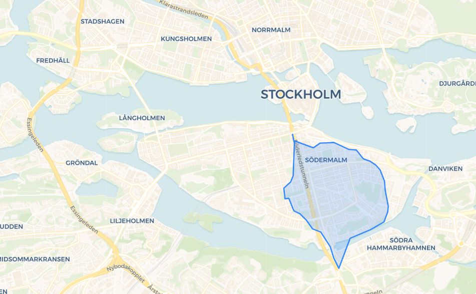
Example of a drive-time analysis conducted using pgrouting (5 min and 10 min walking distance):

This tutorial does not intend to give an extensive guide to install and setup each software as there are many flavors to that and much better tutorials existing (some of which are linked to in this tutorial). Instead, it aims to fill the gap of going from A to B of enabling analysis on road data in a fully open-source way, available for anyone.

Setup

Start by installing PostgreSQL and pgAdmin (if you don’t have it already).

Tutorials for installing PostgreSQL and pgAdmin can for example be found here.

Create your database using psql terminal

When you have installed PostgreSQL it is time to set up your database with its required extensions for road data. Pgrouting is the extension which enables setting up a road network database (you can read more about this here). In turn Pgrouting makes use of another extension called PostGIS. PostGIS is an extension for PostgreSQL for spatial data structures (you can read more about this here).

In psql terminal:

CREATE DATABASE city_routing; ^

connect city_routing;

CREATE EXTENSION pgrouting CASCADE;

This tutorial explains the steps taken to set up and verify the pgrouting database in more detail.

OpenStreetMap road network

Download OpenStreetMap

There are several ways to download OSM data, you can read more about it here. For this tutorial, I’ve used Geofabrik as the source for downloading OSM data as they provide an easy distribution of it. I downloaded the road network of the entire Sweden here as Sweden-latest.osm.bz2. Be aware that the files can be rather large (the zipped file of Sweden is 1GB and unzipped it is 11GB). Unzip the .bz2 file using 7-zip or any other compatible software.

Prepare the data

In this tutorial I’ve used osm2pgrouting as the tool to load the data into the database (It will be further explained later). osm2pgrouting is quick but loads all data into memory which may result in OOM Error if your dataset is too big. There are alternative tools to use such as osm2pgsql or osm2po to bypass this issue. I decided to limit my dataset to Sweden’s capital city, Stockholm, so before loading the dataset I clipped it.

For this, Osmosis software was used, installation and configuration can be found here. You need to either add Osmosis to your environmental variables or run the command from the bin folder of Osmosis (In my case I cd to C:\YourPath\osmosis-0.48.3\bin). To read more about Osmosis go here.

Osmosis command for clipping using a bounding box:

osmosis –read-xml C:\YourPath\sweden-latest.osm –bb left=17.9563 right=18.1481 ^

top=59.3584 bottom=59.286 completeWays=yes –write-xml stockholm.osm

If you would like to clip the dataset using a custom polygon you would have to convert it to a .POLY file, you can read more about this here. If you are familiar with Python, you could use this function.

Osmosis command for clipping using a polygon (this .poly file was generated using the Python function above):

osmosis –read-xml C:\YourPath\sweden-latest.osm –bounding-polygon file=stockholm.poly ^

        completeWays=yes –write-xml stockholm.osm

After this a new .osm file has been produced which covers your area of interest. Now it’s time to push the data into your pgrouting database.

osm2pgrouting

Cd (change directory) in your command prompt to the directory of your .osm file or write out the entire path under the -f statement.

osm2pgrouting command:

osm

osm2pgrouting ^

-c “C:\Program Files\PostgreSQL\13\bin\mapconfig.xml” ^

-f stockholm.osm ^

-d city_routing ^

-U postgres ^

-W YourPassWord ^

    –clean

Now you should have your very own pgrouting database, let’s test it!

Open pgAdmin and run the following queries

The queries below are modifications of example SQL queries found in documentation and other resources found online such as this and Anita Grasers extensive examples on pgrouting.

Query to test shortest distance using Dijkstra’s algorithm on two coordinates:

with source_tmp AS (SELECT source 

            FROM ways 

            ORDER BY st_distance(the_geom, 

                ST_SetSRID(ST_MakePoint(18.01476, 59.32903), 4326)) limit 1),

     target_tmp AS (SELECT target 

            FROM ways 

            ORDER BY st_distance(the_geom, 

                ST_SetSRID(ST_MakePoint(18.0833, 59.3108), 4326)) limit 1)

SELECT * 

FROM pgr_dijkstra(‘SELECT gid AS id

                  , source

                  , target

                  , cost

                  , reverse_cost 

                  FROM ways’

                  , (SELECT source from source_tmp) 

                  , (SELECT target from target_tmp), true) AS r 

LEFT JOIN ways AS w 

ON r.edge = w.gid;

Expected output:

Query to select the roads reachable of 15-minute walking distance (900 seconds):

SELECT ‘Nytorget’ AS name,

        15 AS drive_time,

        ST_Collect(ways.the_geom) AS the_geom 

        FROM ways

    JOIN (SELECT * FROM pgr_drivingDistance(

        ‘SELECT gid AS id

        , source

        , target

        , length_m AS cost 

        FROM “ways”      ‘

        ,53588,900,FALSE) — “53588” is the source vertex of a road segment from which we calculate the driving distance.

) AS route 

  ON ways.target = route.node

Query to create isochrone of 15-minute walking distance (900 seconds):

SELECT ‘Nytorget’ AS name,

        15 AS drive_time,

        ST_CollectionExtract(ST_ConcaveHull(ST_Collect(ways.the_geom), 0.99),3) AS the_geom

        FROM ways

    JOIN (SELECT * FROM pgr_drivingDistance(

        ‘SELECT gid AS id

        , source

        , target

        , length_m AS cost 

        FROM “ways”      ‘

        ,53588,900,FALSE) — “53588” is the source vertex of a road segment from which we calculate the driving distance.

) AS route 

  ON ways.target = route.node

Expected output: